Exploring Global Fertility: A Journey Across Borders
This is a test post. In this post, I try out different functionalities
123
Second Tag
Author
Alex Labuda
Published
December 25, 2023
Let’s Explore the World Ferility Rates
In a world bustling with over seven billion people, each individual represents a unique thread in the intricate tapestry of humanity. But beyond the surface of bustling streets and crowded cities lies a story told not through words, but through numbers - the story of fertility rates. This vital statistic, often overlooked, serves as a silent narrator of our times, speaking volumes about societal trends, economic conditions, and cultural shifts.
As we embark on a journey across continents, we delve into the fascinating world of fertility rates. From the snow-capped villages of Scandinavia to the sun-drenched lands of Sub-Saharan Africa, we’ll explore how these numbers shape nations, influence policies, and reflect the diverse tapestry of human existence.
Join me as we unravel the tales hidden within these figures, discovering not just the “how” and “what,” but the profound “why” behind the fertility rates of various countries. We’ll look at how these rates are more than just numbers on a page; they are a reflection of healthcare access, gender equality, economic stability, and cultural norms.
Through this exploration, we’ll gain a deeper understanding of our world and its future, one number at a time.
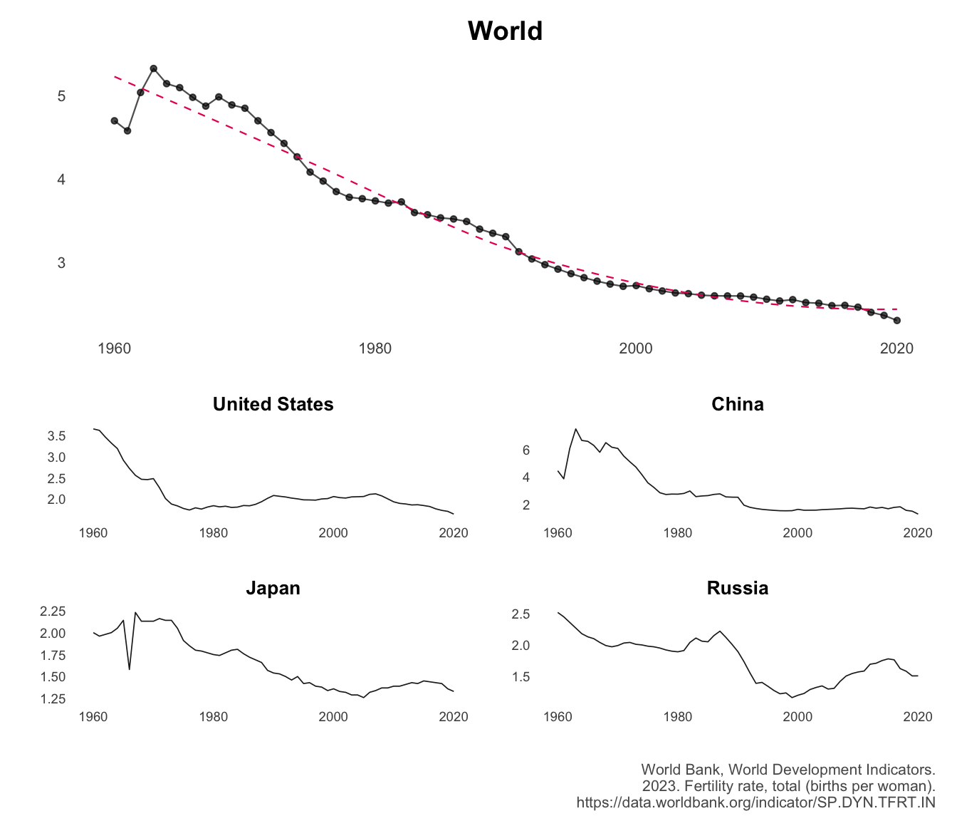
Plot the US birthrates through time
Show the code
# Create a function of the above plot codeplot_line <-function(data, iso2c ="US", title ="United States",title_size =10, hjust =0,dot_size =0.6, linewidth =0.2) {# Check if required columns exist in the dataif (!("iso2c"%in%names(data)) ||!("date"%in%names(data)) ||!("SP.DYN.TFRT.IN"%in%names(data))) {stop("Data must contain 'iso2c', 'date', and 'SP.DYN.TFRT.IN' columns.") }# Filtering and plotting plot <- data %>%filter(iso2c ==!!iso2c) %>%# Correct filteringggplot(aes(x = date, y = SP.DYN.TFRT.IN)) +geom_line(alpha =0.7, linewidth = linewidth) +geom_point(size = dot_size, alpha =0.7) +geom_smooth(span =0.9,linewidth = linewidth,linetype =2,se =FALSE,color ="#E91E63" ) +labs(x ="",y ="",title = title ) +theme(plot.title =element_text(size = title_size, face ="bold",hjust = hjust),axis.title =element_text(size =8, face ="bold"),axis.text =element_text(size =8),legend.position ="none",panel.grid =element_blank() )return(plot)}plot_line_small <-function(data, iso2c ="US", title ="United States",title_size =10, hjust =0,dot_size =0.6, linewidth =0.3) {# Check if required columns exist in the dataif (!("iso2c"%in%names(data)) ||!("date"%in%names(data)) ||!("SP.DYN.TFRT.IN"%in%names(data))) {stop("Data must contain 'iso2c', 'date', and 'SP.DYN.TFRT.IN' columns.") }# Filtering and plotting plot <- data %>%filter(iso2c ==!!iso2c) %>%# Correct filteringggplot(aes(x = date, y = SP.DYN.TFRT.IN)) +geom_line(alpha =0.9, linewidth = linewidth) +# geom_point(size = dot_size, alpha = 0.7) +# geom_smooth(# span = 0.9,# linewidth = linewidth,# linetype = 2,# se = FALSE,# color = "#E91E63"# ) +labs(x ="",y ="",title = title ) +theme(plot.title =element_text(size = title_size, face ="bold",hjust = hjust),axis.title =element_text(size =8, face ="bold"),axis.text =element_text(size =7),legend.position ="none",panel.grid =element_blank() )return(plot)}